Caleb Williams Looks Bad Until You Look Closer
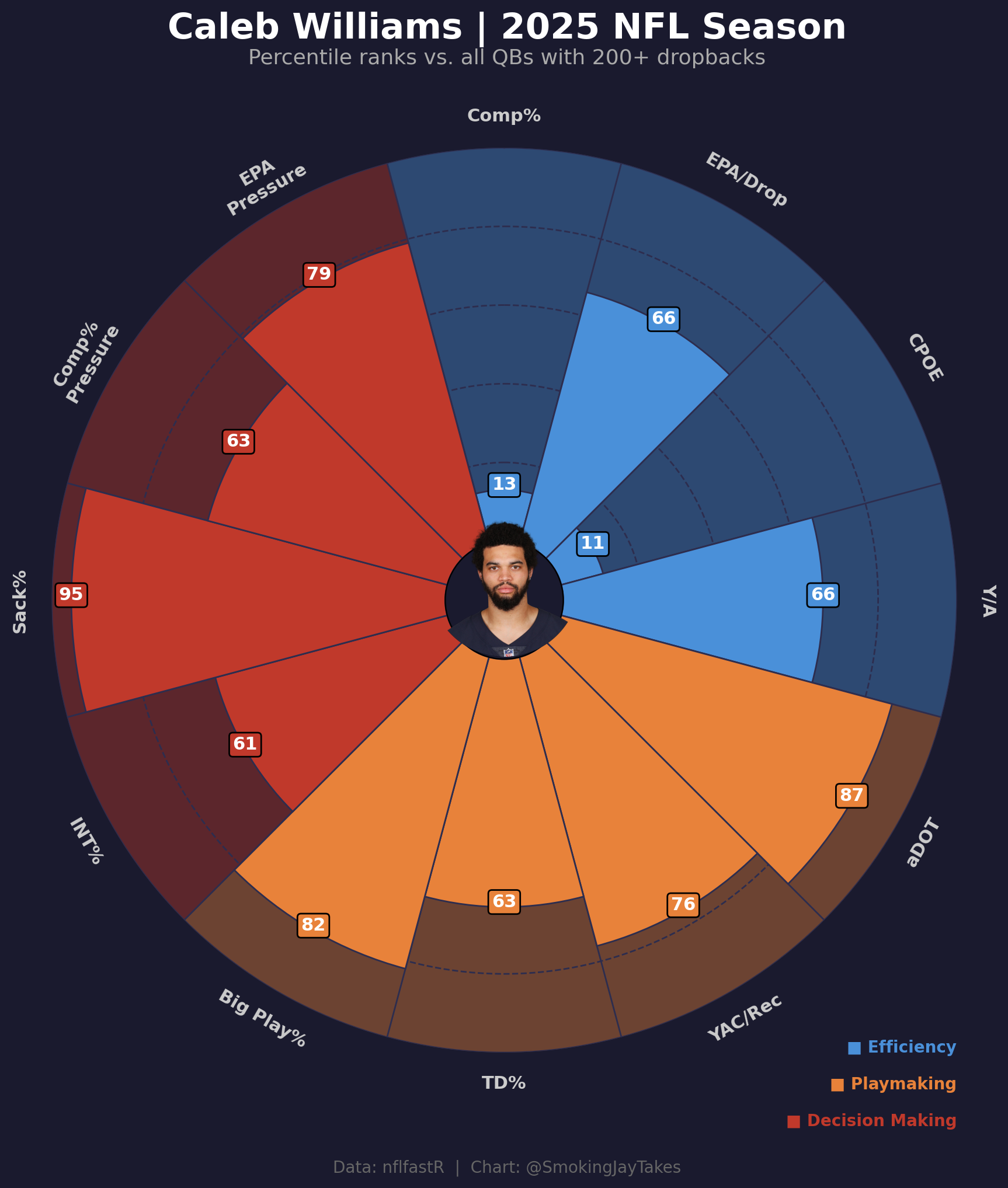
A pizza chart of Caleb's 2025 percentile ranks tells a more complicated story than the raw stats let on. I built the viz with Python and mplsoccer, and the numbers were surprising.
Caleb Williams’ 2025 season is pretty difficult to evaluate if you only look at the most common efficiency stats.
Among qualifying quarterbacks, Caleb finished in the 13th percentile in completion percentage and the 11th percentile in CPOE. Those are obviously poor numbers. CPOE is especially important here because it accounts for the difficulty of each throw, so this is not just a case of Caleb having a lower completion percentage because he was throwing the ball further downfield. Even after adjusting for throw difficulty, he was still near the bottom of the league.
However, when looking at his full percentile profile across 12 different metrics, the picture becomes a lot more interesting.
I created a pizza chart separating the metrics into three general categories: efficiency, playmaking, and decision making. Each slice shows Caleb’s percentile rank compared to quarterbacks with at least 200 dropbacks during the 2025 season.
The efficiency profile is uneven
The first thing that stands out is how uneven the efficiency profile is. His completion percentage and CPOE are both extremely low, but his EPA per dropback and yards per attempt are both in the 66th percentile. This means that while Caleb was missing more throws than expected, the offense was still generating above-average value on his dropbacks. A lot of that appears to come from the type of throws he was attempting and the value created when those throws connected.
The playmaking profile is much stronger
His playmaking numbers were much stronger. Caleb ranked in the 87th percentile in aDOT, which shows how aggressive he was in pushing the ball downfield. He also ranked in the 82nd percentile in big play rate, the 76th percentile in yards after catch per reception, and the 63rd percentile in touchdown rate.
This explains a lot of the tension in his profile. The low completion numbers are real, but they came alongside a very aggressive downfield passing approach. Caleb was not building his statistical profile through short, easy throws. He was consistently attacking deeper areas of the field, and when those plays worked, they created real value for the offense.
Sack avoidance and pressure performance matter here
The sack rate number was the most surprising part of the chart. Caleb ranked in the 95th percentile in sack rate, meaning he was one of the best quarterbacks in the league at avoiding sacks. Given how often the conversation around him focuses on holding the ball too long or creating pressure on himself, this was an important finding. Whatever issues existed in the passing game, taking sacks was not one of the main ones in 2025.
His numbers under pressure were also strong. Caleb ranked in the 79th percentile in EPA under pressure and the 63rd percentile in completion percentage under pressure. Those are both above-average marks and suggest that his production did not fall apart when the pocket got messy.
The bigger takeaway
Overall, Caleb’s 2025 profile is hard to summarize cleanly. The accuracy concerns are real, especially with an 11th percentile CPOE. That cannot just be ignored or explained away. At the same time, the rest of the profile shows a quarterback who created explosive plays, pushed the ball downfield, avoided sacks at an elite rate, and still produced above-average value per dropback.
The biggest question going forward is whether he can improve the accuracy while keeping the parts of his game that already create value. If the CPOE stays this low, it will cap the offense. But if that number improves, the rest of the profile already points to a quarterback with a lot of valuable traits.
The chart does not give a final answer on Caleb. It mostly shows why the conversation around him should be more specific. Completion percentage and CPOE tell an important part of the story, but they do not explain the whole season.
How I built it
The whole thing runs on nfl_data_py for the play-by-play and mplsoccer's PyPizza for the visualization. Headshot pulls straight from the nflverse roster parquet.
Data pipeline
First, pull play-by-play and find Caleb's gsis_id:
import nfl_data_py as nflimport pandas as pd pbp = nfl.import_pbp_data([2025]) rosters = pd.read_parquet( "https://github.com/nflverse/nflverse-data/releases/download/rosters/roster_2025.parquet") caleb_roster = rosters[ (rosters['full_name'].str.contains('Caleb Williams', case=False, na=False)) & (rosters['team'] == 'CHI')]caleb_id = caleb_roster.iloc[0]['gsis_id']headshot_url = caleb_roster.iloc[0]['headshot_url']Then filter to QBs with 200+ dropbacks and compute the metrics:
from scipy.stats import percentileofscoreimport numpy as np dropbacks = pbp[pbp['qb_dropback'] == 1].copy()dropback_counts = dropbacks.groupby('passer_player_id').size().reset_index(name='dropbacks')qualifying_qbs = dropback_counts[dropback_counts['dropbacks'] >= 200]['passer_player_id'].tolist() pass_plays = pbp[(pbp['pass_attempt'] == 1) & (pbp['two_point_attempt'] == 0)].copy()For each qualifying QB I compute 12 stats: comp%, EPA/dropback, CPOE, Y/A, aDOT, YAC/rec, TD%, big play%, INT%, sack%, comp% under pressure, and EPA under pressure. Two of them (INT% and sack%) are inverted before percentile ranking so higher is always better.
metrics = [ ('comp_pct', 'Comp%', False), ('epa_dropback', 'EPA/Drop', False), ('cpoe', 'CPOE', False), ('yards_att', 'Y/A', False), ('adot', 'aDOT', False), ('yac_rec', 'YAC/Rec', False), ('td_pct', 'TD%', False), ('big_play_pct', 'Big Play%', False), ('int_pct', 'INT%', True), # lower is better → invert ('sack_pct', 'Sack%', True), # lower is better → invert ('comp_under_pressure', 'Comp%\nPressure', False), ('epa_under_pressure', 'EPA\nPressure', False),] values = []for col, label, inverted in metrics: raw_val = caleb[col] col_vals = qb_df[col].dropna().values pct = percentileofscore(col_vals, raw_val) if inverted: pct = 100 - pct values.append(round(pct))Building the pizza
PyPizza handles most of the heavy lifting. I passed three slice colors to separate the metric groups visually:
from mplsoccer import PyPizza slice_colors = [ "#4A90D9", "#4A90D9", "#4A90D9", "#4A90D9", # efficiency "#E8823A", "#E8823A", "#E8823A", "#E8823A", # playmaking "#C0392B", "#C0392B", "#C0392B", "#C0392B", # decision making] baker = PyPizza( params=params, background_color="#1A1A2E", straight_line_color="#2D2D4E", straight_line_lw=1, last_circle_color="#2D2D4E", last_circle_lw=1, other_circle_color="#2D2D4E", other_circle_lw=1, inner_circle_size=15,) fig, ax = baker.make_pizza( values, figsize=(10, 10.5), color_blank_space="same", slice_colors=slice_colors, value_colors=["#FFFFFF"] * 12, value_bck_colors=slice_colors, blank_alpha=0.4, kwargs_slices=dict(edgecolor="#2D2D4E", zorder=2, linewidth=1), kwargs_params=dict(color="#CCCCCC", fontsize=11, fontweight="bold", va="center"), kwargs_values=dict( color="#FFFFFF", fontsize=11, fontweight="bold", bbox=dict(edgecolor="#000000", boxstyle="round,pad=0.2", lw=1) ),)The headshot goes in the center using ax.inset_axes. Getting it to sit exactly at the pizza's center took some fiddling (the axes center and the pizza center don't perfectly overlap):
from PIL import Image, ImageDrawfrom io import BytesIOfrom urllib.request import urlopenimport numpy as np response = urlopen(headshot_url)img = Image.open(BytesIO(response.read())) # Circular cropsize = min(img.size)mask = Image.new('L', (size, size), 0)draw = ImageDraw.Draw(mask)draw.ellipse((0, 0, size, size), fill=255) left = (img.width - size) // 2top = (img.height - size) // 2img_cropped = img.crop((left, top, left + size, top + size))img_cropped = img_cropped.convert('RGBA') circ_headshot = Image.new('RGBA', (size, size), (0, 0, 0, 0))circ_headshot.paste(img_cropped, mask=mask) # Place at pizza centerpizza_cx, pizza_cy = 0.5, 0.52img_frac = 0.165 ax_img = ax.inset_axes( [pizza_cx - img_frac / 2, pizza_cy - img_frac / 2, img_frac, img_frac])ax_img.imshow(np.array(circ_headshot))ax_img.axis("off")ax_img.set_zorder(5)Data from nflfastR via nfl_data_py. Full script on my GitHub.